Appearance
PyTorchBlitz学习笔记
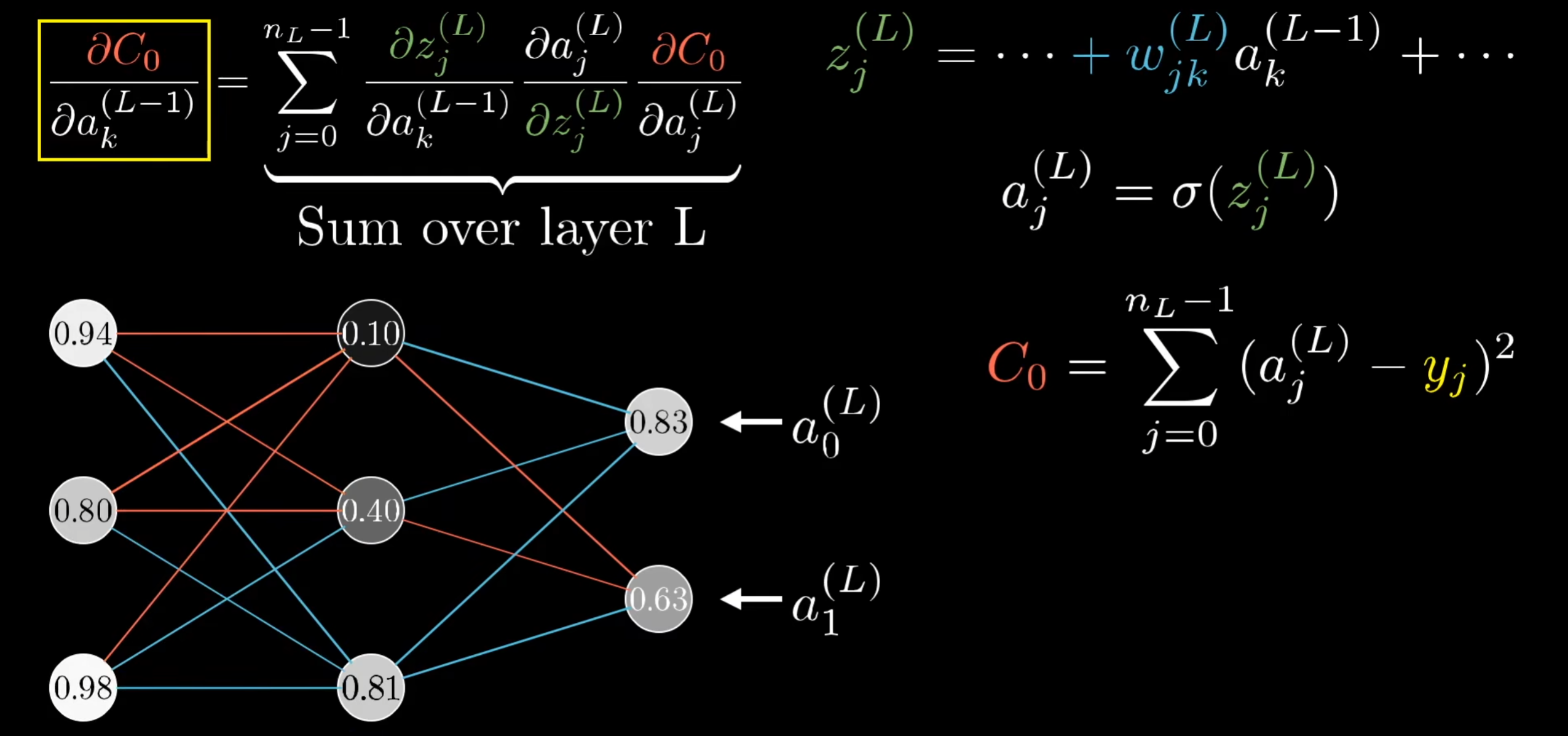
以下为 3b1b 中有关反向传播算法原理的介绍 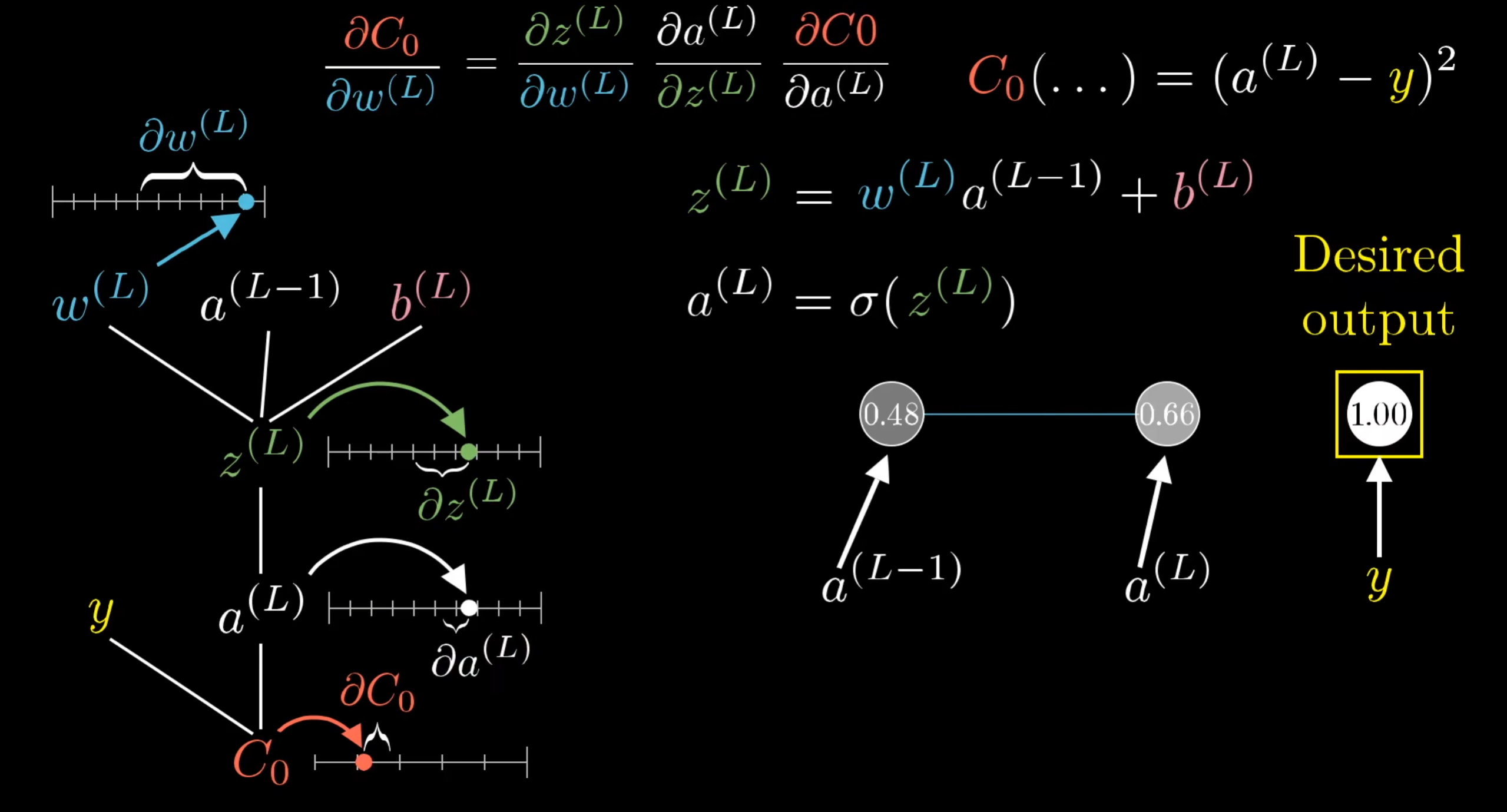
torch.autograd 简介
在对 Tensor 做操作时,autograd 会记录其输入张量与输出张量,并构建一个有向无环图(DAG)[1],其中根为输入张量,叶子为输出张量。在反向传递时调用.backward()时,autograd 会从每个.grad_fn 计算梯度并累积在各自张量的 .grad 属性中,最终传播到叶子即输出张量
python
import torch
from torchvision.models import resnet18, ResNet18_Weights
model = resnet18(weights=ResNet18_Weights.DEFAULT)
data = torch.rand(1, 3, 64, 64)
labels = torch.rand(1, 1000)

prediction = model(data) # 前向传播

loss = (prediction - labels).sum() #某种代价值但不是常用的
loss.backward() #反向传播

#SGD——Stochastic Gradient Descent随机梯度下降
#model.parameters() 模型的权重与偏置
#lr为学习率或者说步长
#momentum为动量,也可以理解为惯性
optim = torch.optim.SGD(model.parameters(), lr=1e-2, momentum=0.9)

optim.step() #梯度下降Autograd 中的自动微分
python
import torch

#创建张量并使用requires_grad追踪操作
#通过requires_grad=True控制张量是否需要进行梯度
a = torch.tensor([2., 3.], requires_grad=True)
b = torch.tensor([6., 4.], requires_grad=True)

Q = 3*a**3 - b**2

external_grad = torch.tensor([1., 1.])
Q.backward(gradient=external_grad)

# 检查结果是否为a与b向量求导后的结果
print(9*a**2 == a.grad)
print(-2*b == b.grad)autograd 追踪计算原理:
神经网络(Neural Networks)
结合 3B1B 视频可以更好理解原理
python
import torch
import torch.nn as nn
import torch.nn.functional as F

class Net(nn.Module):

    def __init__(self):
        super(Net, self).__init__()
        # 1 input image channel, 6 output channels, 5x5 square convolution对应self.conv1
        # 一个输入图像通道,6个输出通道,在5×5的正方形卷积核中
        # 卷积层self.conv
        self.conv1 = nn.Conv2d(1, 6, 5)
        self.conv2 = nn.Conv2d(6, 16, 5)
        # 连接层self.fc
        # an affine operation: y = Wx + b(权重×特征+偏置)
        self.fc1 = nn.Linear(16 * 5 * 5, 120)  # 5*5 from image dimension
        self.fc2 = nn.Linear(120, 84)
        self.fc3 = nn.Linear(84, 10)

    def forward(self, input):
        # Convolution layer C1: 1 input image channel, 6 output channels,
                # 5x5 square convolution, it uses RELU activation function, and        # outputs a Tensor with size (N, 6, 28, 28), where N is the size of the batch        # 特征提取
        # 卷积层c1,将图像输出为(N, 6, 28, 28)的格式,后续c3为第二个卷积层
        c1 = F.relu(self.conv1(input))
        # Subsampling layer S2: 2x2 grid, purely functional,
        # this layer does not have any parameter, and outputs a (N, 6, 14, 14) Tensor        # 下采样/池化层,长宽各缩减一半(特征浓缩),后续s4为第二次最大池化
        s2 = F.max_pool2d(c1, (2, 2))
        # Convolution layer C3: 6 input channels, 16 output channels,
        # 5x5 square convolution, it uses RELU activation function, and        # outputs a (N, 16, 10, 10) Tensor
        c3 = F.relu(self.conv2(s2))
        # Subsampling layer S4: 2x2 grid, purely functional,
        # this layer does not have any parameter, and outputs a (N, 16, 5, 5) Tensor        s4 = F.max_pool2d(c3, 2)
        # Flatten operation: purely functional, outputs a (N, 400) Tensor
        # 展平,将多维图像拉直为一维向量
        s4 = torch.flatten(s4, 1)
        # Fully connected layer F5: (N, 400) Tensor input,
        # and outputs a (N, 120) Tensor, it uses RELU activation function        # 分类决策
        f5 = F.relu(self.fc1(s4))
        # Fully connected layer F6: (N, 120) Tensor input,
        # and outputs a (N, 84) Tensor, it uses RELU activation function
        f6 = F.relu(self.fc2(f5))
        # Fully connected layer OUTPUT: (N, 84) Tensor input, and
        # outputs a (N, 10) Tensor        # 输出最终输出 10个分类的得分
        output = self.fc3(f6)
        return output

net = Net()
print(net)
# 模型的学习参数
params = list(net.parameters())
print(len(params)) # 2个卷积层 + 3个全连接层,每一层两种参数——权重(Weight)×偏置(Bias)=10
print(params[0].size())  # conv1's .weight [输出通道数, 输入通道数, 卷积核高度, 卷积核宽度]—
                        # 输出通道数:卷积核数目,输入通道数:黑白图片只有1个通道,卷积核尺寸:5, 5

#随机的32×32输入到神经网络
input = torch.randn(1, 1, 32, 32)
out = net(input)
print(out)
#反向传播
net.zero_grad()
out.backward(torch.randn(1, 10))

# NN包中的损失函数
output = net(input)
target = torch.randn(10)  # a dummy target, for example
target = target.view(1, -1)  # make it the same shape as output
criterion = nn.MSELoss() #MSE:输出与目标均方差

loss = criterion(output, target) # 损失函数
print(loss)

# 反向传播
net.zero_grad()     # zeroes the gradient buffers of all parameters

print('conv1.bias.grad before backward')
print(net.conv1.bias.grad)

loss.backward()

print('conv1.bias.grad after backward')
print(net.conv1.bias.grad)

# 更新权重
# weight = weight - learning_rate * gradient 权重-学习率×梯度
learning_rate = 0.01
for f in net.parameters():
f.data.sub_(f.grad.data * learning_rate)训练图像分类器(Training a Classifier)
神经网络训练循环流程图如图(ChatGPT生成): 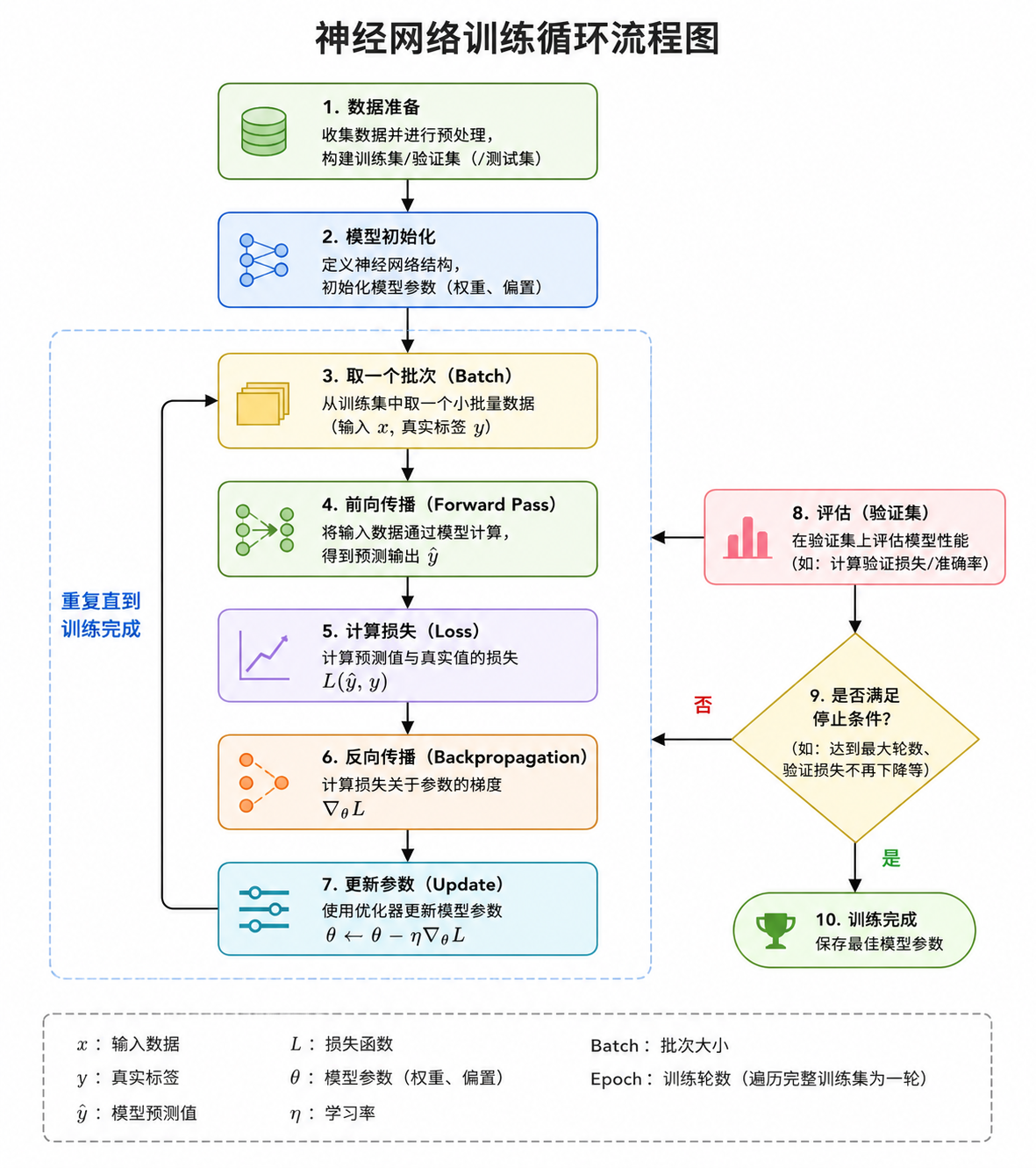 在官网给的代码中
num_workers=2在Windows系统会导致死循环,解决方法是将训练代码全部放在if __name__ == '__main__':下,或直接更改num_workers=0[2]
python
import torch
import torch.nn as nn
import torch.nn.functional as F
import torch
import torchvision
import torchvision.transforms as transforms
import torch.optim as optim
class Net(nn.Module):
def __init__(self):
super().__init__()
self.conv1 = nn.Conv2d(3, 6, 5)
self.pool = nn.MaxPool2d(2, 2)
self.conv2 = nn.Conv2d(6, 16, 5)
self.fc1 = nn.Linear(16 * 5 * 5, 120)
self.fc2 = nn.Linear(120, 84)
self.fc3 = nn.Linear(84, 10)
def forward(self, x):
x = self.pool(F.relu(self.conv1(x)))
x = self.pool(F.relu(self.conv2(x)))
x = torch.flatten(x, 1) # flatten all dimensions except batch
x = F.relu(self.fc1(x))
x = F.relu(self.fc2(x))
x = self.fc3(x)
return x
net = Net()
if __name__ == '__main__':
transform = transforms.Compose(
[transforms.ToTensor(), # 将图片转化为张量并进行归一化
transforms.Normalize((0.5, 0.5, 0.5), (0.5, 0.5, 0.5))]) # 将RGB颜色进行标准化
batch_size = 4 # 每次训练数据个数
trainset = torchvision.datasets.CIFAR10(root='./data', train=True,
download=True, transform=transform) # 数据集
trainloader = torch.utils.data.DataLoader(trainset, batch_size=batch_size,
shuffle=True, num_workers=10)
# 数据搬运,batch_size每次搬运数据数,shuffle数据顺序打乱,num_workers并行线程
# 训练集
testset = torchvision.datasets.CIFAR10(root='./data', train=False,
download=True, transform=transform)
testloader = torch.utils.data.DataLoader(testset, batch_size=batch_size,
shuffle=False, num_workers=10)
# 训练后对应的标签
classes = ('plane', 'car', 'bird', 'cat',
'deer', 'dog', 'frog', 'horse', 'ship', 'truck')
import matplotlib.pyplot as plt
import numpy as np
# functions to show an image
def imshow(img):
img = img / 2 + 0.5 # unnormalize
npimg = img.numpy()
plt.imshow(np.transpose(npimg, (1, 2, 0)))
plt.show()
# get some random training images
# 获取随机训练数据
dataiter = iter(trainloader)
images, labels = next(dataiter)
# 展示图片
imshow(torchvision.utils.make_grid(images))
# 输出标签
print(' '.join(f'{classes[labels[j]]:5s}' for j in range(batch_size)))
#定义损失函数和优化器
criterion = nn.CrossEntropyLoss()
optimizer = optim.SGD(net.parameters(), lr=0.001, momentum=0.9)
#训练网路
for epoch in range(2): # loop over the dataset multiple times
running_loss = 0.0
for i, data in enumerate(trainloader, 0):
# get the inputs; data is a list of [inputs, labels]
inputs, labels = data
# zero the parameter gradients
optimizer.zero_grad()
# forward + backward + optimize
outputs = net(inputs)
loss = criterion(outputs, labels)
loss.backward()
optimizer.step()
# print statistics
running_loss += loss.item()
if i % 2000 == 1999: # print every 2000 mini-batches
print(f'[{epoch + 1}, {i + 1:5d}] loss: {running_loss / 2000:.3f}')
running_loss = 0.0
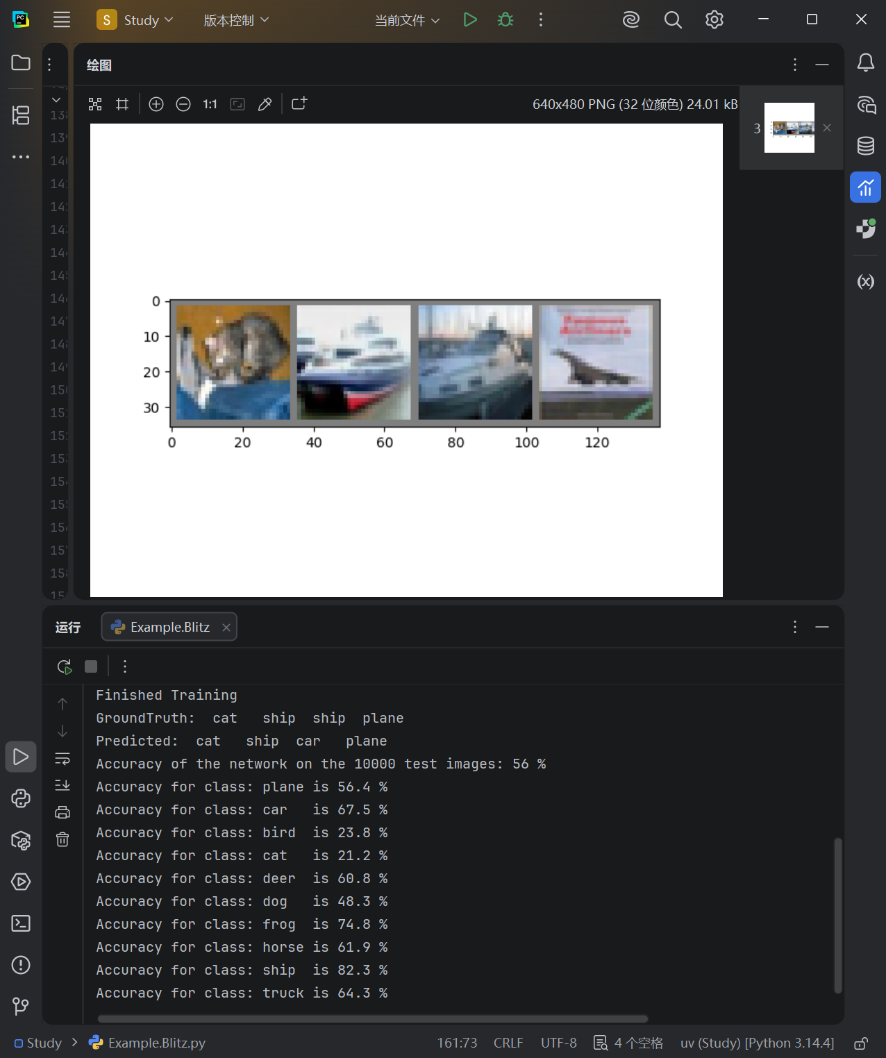
print('Finished Training')
#保存模型
PATH = './cifar_net.pth'
torch.save(net.state_dict(), PATH)
#进行测试
dataiter = iter(testloader)
images, labels = next(dataiter)
# print images
imshow(torchvision.utils.make_grid(images))
print('GroundTruth: ', ' '.join(f'{classes[labels[j]]:5s}' for j in range(4)))
net = Net()
net.load_state_dict(torch.load(PATH, weights_only=True))
outputs = net(images) #神经网络识别结果
_, predicted = torch.max(outputs, 1)
#图像预测结果
print('Predicted: ', ' '.join(f'{classes[predicted[j]]:5s}'for j in range(4)))
#整体数据集表现
correct = 0
total = 0
# since we're not training, we don't need to calculate the gradients for our outputs
with torch.no_grad():
for data in testloader:
images, labels = data
# calculate outputs by running images through the network
outputs = net(images)
# the class with the highest energy is what we choose as prediction
_, predicted = torch.max(outputs, 1)
total += labels.size(0)
correct += (predicted == labels).sum().item()
print(f'Accuracy of the network on the 10000 test images: {100 * correct // total} %')
#具体每类表现
# prepare to count predictions for each class
correct_pred = {classname: 0 for classname in classes}
total_pred = {classname: 0 for classname in classes}
# again no gradients needed
with torch.no_grad():
for data in testloader:
images, labels = data
outputs = net(images)
_, predictions = torch.max(outputs, 1)
# collect the correct predictions for each class
for label, prediction in zip(labels, predictions):
if label == prediction:
correct_pred[classes[label]] += 1
total_pred[classes[label]] += 1
# print accuracy for each class
for classname, correct_count in correct_pred.items():
accuracy = 100 * float(correct_count) / total_pred[classname]
print(f'Accuracy for class: {classname:5s} is {accuracy:.1f} %')最终训练结果如图: